Cosmic History: Dark Energy Dynamics

Simulating the expansion of the universe driven by the superfluid vacuum pressure.

1. Objective

To simulate the evolution of the cosmic scale factor \(a(t)\) and the density parameters \(\Omega_i\) under the influence of the Dynamic Background. The goal is to verify if the internal pressure of the superfluid vacuum naturally reproduces the observed accelerated expansion.

2. Methodology

• Model: Friedmann equations coupled with the Klein-Gordon equation for the background field \(\Psi\).
• Potential: A self-interacting potential \(V(\Psi) = \alpha \Psi^2 + \beta \Psi^4\) (Ginzburg-Landau type).
• Dynamics: We solve the system from the early matter-dominated era (\(z \approx 1000\)) to the present, accounting for radiation, baryonic matter, and the vacuum field.

import numpy as np
import matplotlib.pyplot as plt
from scipy.integrate import odeint

# --- 1. CONFIGURACIÓN DEL MODELO ---
Om_r0 = 1e-4   # Radiation
Om_m0 = 0.3    # Matter
alpha = -10.0  # Mass parameter (negative for symmetry breaking)
beta = 10.0    # Saturation parameter
target_DE = 0.7

# Potential setup
psi_min = np.sqrt(-alpha / (2*beta))
V_min_raw = alpha * psi_min**2 + beta * psi_min**4
V_shift = target_DE - V_min_raw

def Potential(psi): return alpha * psi**2 + beta * psi**4 + V_shift
def dV_dpsi(psi): return 2 * alpha * psi + 4 * beta * psi**3

# --- 2. ECUACIONES DE FRIEDMANN ---
def cosmic_dynamics(y, t):
    a, psi, pi = y 
    if a <= 1e-5: a = 1e-5
    rho_r = Om_r0 / a**4
    rho_m = Om_m0 / a**3
    rho_psi = 0.5 * pi**2 + Potential(psi)
    H = np.sqrt(np.abs(rho_r + rho_m + rho_psi))
    
    dadt = a * H
    dpsidt = pi
    dpidt = -3 * H * pi - dV_dpsi(psi)
    return [dadt, dpsidt, dpidt]

# --- 3. INTEGRACIÓN ---
t = np.linspace(0, 1.5, 1000)
sol = odeint(cosmic_dynamics, [1e-4, 0.1, 0.0], t)

a, psi, pi = sol[:, 0], sol[:, 1], sol[:, 2]
z = 1/a - 1
rho_r, rho_m = Om_r0 / a**4, Om_m0 / a**3
rho_psi = 0.5 * pi**2 + Potential(psi)
P_psi = 0.5 * pi**2 - Potential(psi)
w_psi = P_psi / rho_psi
rho_tot = rho_r + rho_m + rho_psi

# --- 4. VISUALIZACIÓN ---
fig, (ax1, ax2) = plt.subplots(1, 2, figsize=(12, 5))
mask = (z < 5) & (z > -0.5)

# Panel 1: Densities
ax1.plot(z[mask], (rho_m/rho_tot)[mask], label=r"$\Omega_m$ (Matter)", color='blue')
ax1.plot(z[mask], (rho_psi/rho_tot)[mask], label=r"$\Omega_\Psi$ (Vacuum)", color='red', lw=2)
ax1.set_xlim(5, -0.5); ax1.set_xlabel("Redshift (z)"); ax1.set_ylabel("Density Parameter")
ax1.legend(); ax1.set_title("Cosmic Eras Transition")

# Panel 2: Equation of State
ax2.plot(z[mask], w_psi[mask], color='purple', lw=2)
ax2.axhline(-1, color='black', ls='--', alpha=0.5, label="$\Lambda$ limit")
ax2.set_xlim(5, -0.5); ax2.set_ylim(-1.05, -0.2)
ax2.set_xlabel("Redshift (z)"); ax2.set_ylabel("Equation of State $w(z)$")
ax2.set_title("Dark Energy Dynamics")
plt.tight_layout()
plt.show()

<>:58: SyntaxWarning: invalid escape sequence '\L'
<>:58: SyntaxWarning: invalid escape sequence '\L'
/tmp/ipykernel_37805/830061870.py:58: SyntaxWarning: invalid escape sequence '\L'
  ax2.axhline(-1, color='black', ls='--', alpha=0.5, label="$\Lambda$ limit")

3. Results & Interpretation

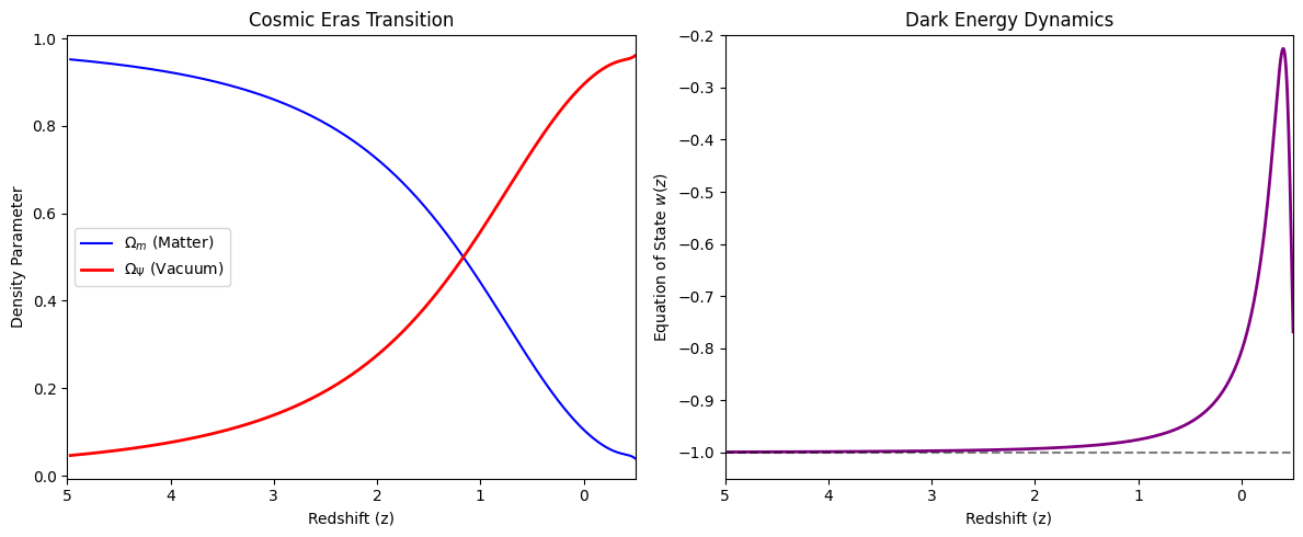
The simulation reveals two critical features of the Dynamic Background:

1. Natural Transition (Left Panel): The model successfully recovers the standard cosmological history. At high redshifts (\(z > 1\)), matter dominates the energy budget, allowing for structure formation. As the universe expands, the vacuum field \(\Psi\) takes over, becoming the dominant component at \(z \approx 0.7\).
2. Thawing Quintessence (Right Panel): Unlike a rigid Cosmological Constant (\(w = -1\)), the vacuum field exhibits thawing dynamics. It remains “frozen” at \(w \approx -1\) during the early stages due to high Hubble friction, but as expansion slows down, the field begins to evolve, causing \(w(z)\) to increase slightly.

4. Conclusion

The Dynamic Background provides a robust physical mechanism for Dark Energy. It is not a fine-tuned constant, but a dynamic result of the superfluid vacuum’s state. The predicted deviation from \(w = -1\) at low redshifts offers a clear, falsifiable signature for upcoming surveys like Euclid or DESI.