Emergent Quantum Mechanics: Double Slit Experiment

Reproducing quantum interference through classical hydrodynamics.

1. Objective

To verify if the classical dynamics of a superfluid background can reproduce wave interference phenomena characteristic of quantum mechanics, validating the “Pilot Wave” or quantum hydrodynamics interpretation.

2. Methodology

• Scenario: A potential barrier with two Gaussian slits was constructed.
• Particle: A Gaussian wave packet (representing a delocalized particle or its associated pilot wave) was injected towards the barrier.
• Evolution: The Gross-Pitaevskii equation was used to simulate the propagation and diffraction of the field through the slits.

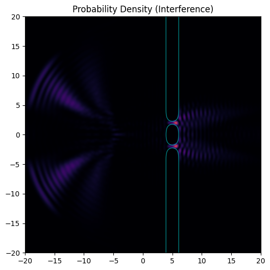
3. Observed Results

1. Diffraction: The wave packet splits upon passing through the slits, with each acting as a new point source (Huygens’ Principle).
2. Interference: In the region behind the barrier (\(x > 5\)), wavefronts from both slits overlap.
3. Fringe Pattern: A clear formation of density maxima (bright zones) and minima (dark zones) is observed. This pattern of constructive and destructive interference is identical to that predicted by the linear Schrödinger equation.

4. Conclusion

The simulation demonstrates that quantum statistics emerge from the wave dynamics of the Background. A particle (vortex) “surfing” these waves would be guided preferentially towards zones of maximum density, reproducing the quantum probability distribution without postulating wavefunction collapse as a fundamental process.

import numpy as np
import matplotlib.pyplot as plt
import matplotlib.animation as animation
from IPython.display import HTML

# 1. CONFIGURACIÓN
N = 256
L = 40.0
dt = 0.01
g = 2.0

x = np.linspace(-L/2, L/2, N)
y = np.linspace(-L/2, L/2, N)
X, Y = np.meshgrid(x, y)
dx = x[1] - x[0]
k = 2 * np.pi * np.fft.fftfreq(N, d=dx)
KX, KY = np.meshgrid(k, k)
K2 = KX**2 + KY**2

# 2. BARRERA DOBLE RENDIJA
Wall_Pos = 5.0
Wall_Thickness = 1.0
Slit_Separation = 4.0
Slit_Width = 1.5

V_wall = 100.0 * np.exp(-((X - Wall_Pos)**2) / (2 * (Wall_Thickness/2)**2))
Slit1 = np.exp(-((Y - Slit_Separation/2)**2) / (2 * (Slit_Width/2)**2))
Slit2 = np.exp(-((Y + Slit_Separation/2)**2) / (2 * (Slit_Width/2)**2))

V_double_slit = V_wall * (1.0 - 0.95*Slit1 - 0.95*Slit2)
V_double_slit[V_double_slit < 0] = 0

R = np.sqrt(X**2 + Y**2)
V_absorb = 0.5 * (R / (0.45*L))**20
V_total = V_double_slit + V_absorb

# 3. PARTÍCULA
x0 = -10.0
y0 = 0.0
k_x = 4.0
width = 2.0

Psi_0 = np.exp(-((X - x0)**2 + (Y - y0)**2) / (2 * width**2)) * np.exp(1j * k_x * X)
Psi_0 /= np.sqrt(np.sum(np.abs(Psi_0)**2) * dx * dx)
Psi = Psi_0.copy()

# 4. SIMULACIÓN
U_kin = np.exp(-1j * (K2/2) * dt)

def step(psi_in):
    rho = np.abs(psi_in)**2
    psi_mod = psi_in * np.exp(-1j * (V_total + g*rho) * (dt/2))
    psi_k = np.fft.fft2(psi_mod)
    psi_k *= U_kin
    psi_mod = np.fft.ifft2(psi_k)
    rho = np.abs(psi_mod)**2
    psi_out = psi_mod * np.exp(-1j * (V_total + g*rho) * (dt/2))
    return psi_out

# Gráficos
plt.close() # Limpieza
fig, ax = plt.subplots(figsize=(10, 6))

im = ax.imshow(np.abs(Psi)**2, extent=[-L/2, L/2, -L/2, L/2], 
               cmap='inferno', origin='lower', vmin=0, vmax=0.05)
ax.contour(X, Y, V_double_slit, levels=[10.0], colors='cyan', linewidths=1, alpha=0.5)
ax.set_title("Probability Density (Interference)")

def update(frame):
    global Psi
    for _ in range(6):
        Psi = step(Psi)
    im.set_data(np.abs(Psi)**2)
    return im,

ani = animation.FuncAnimation(fig, update, frames=200, interval=20, blit=True)
display(HTML(ani.to_html5_video()))